Notes on the Fast.ai Introduction to Machine Learning course
published on December 11th, 2019
In the first seven weeks of my ultralearning data science project, I watched the twelve lectures from the Introduction to Machine Learning for Coders course. Here are my notes on what I learned from this course.
Overview and Summary
The course mostly covers two main topics: random forests and neural networks. I would say that random forests are covered in some depth, for neural networks the course gives a brief introduction into building a simple network for the MNIST dataset and doing some sentiment analysis using logisitic regression.
More than the theoretical models, the course gives a very hands-on approach, immediately jumping into Kaggle competitions and discussing practical aspects of data science / machine learning such as the importance of picking a good validation set or ways to wrangle data using the pandas library. This I would say is the big value of the course: it doesn't spent time on theoretical concepts not really needed for practical work but dives right in. This comes at the expense of glossing over a lot of concepts and risks giving a very superficial understanding, but it firmly maintains the goal of getting the student ready to apply the models right away and build understanding once some practical results have been achieved. What is also great is that the course encourages practical applications ("submit to Kaggle every day") and actively publishing ones learnings which of course bodes very well with the ultralearning principles.
In a little more detail, the course covers the following topics and aspects:
- Random Forests: How to use them, how they work, how to interpret them and where they are limited.
- Neural Nets: Brief application to MNIST, gradient descent & stochastic gradient descent, how to do this with pytorch and what is under the highest level of abstractions, a brief look at embedding matrices and application to structured data problems.
- Practical Advice: Importance of a good validation set and some advice on how to do this, subsampling data to keep things performant, overparameterizing models and using regularization instead of using more restricted models, fitting parameters instead of relying on theoretical parameter sets, doing exploratory data analysis and some feature engineering.
- Sentiment Analysis in NLP using naïve Bayes and the term-document matrix as well as logistic regression.
- Python basics and scientific programming concepts such as vectorized computations and broadcasting, OOP.
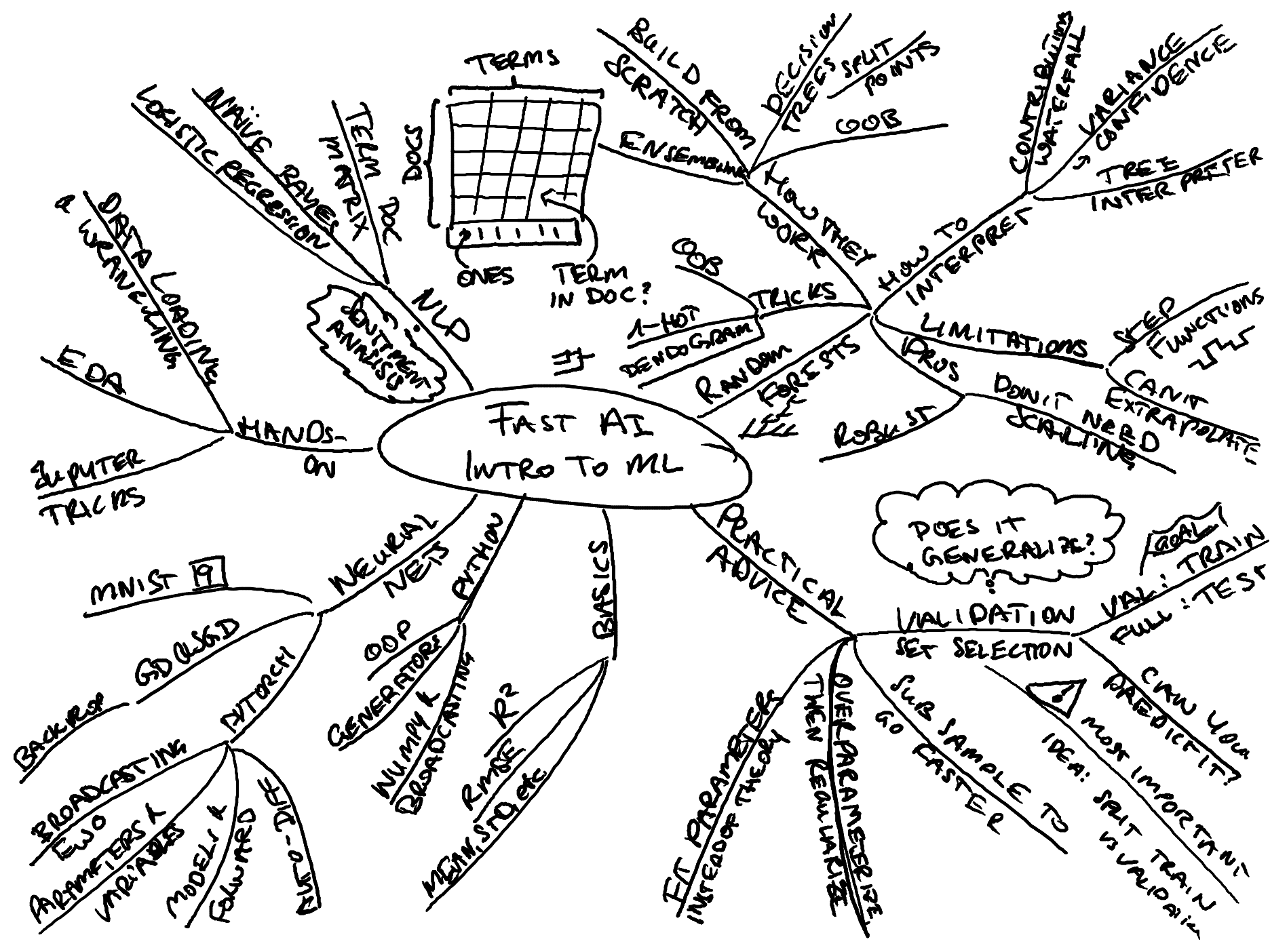
Here is my mindmap overview over the topics covered in this course:
A strength of the course is that it approaches the whole subject from a very pragmatic angle and tries to de-complicate and de-mystify things where it can. It does what it can to make topic accessible. It touches on a ton of small things that arise in practice which more theoretical courses never really get into and which can make progress difficult initially.
A weakness of the course is that it seems unstructured and chaotic jumping across and touching on many topics very briefly to then go elsewhere. Overall, one could say there is not that much ground covered given the time of the lectures.
1. Random Forests
Intro to Random Forests
A decision tree is a simple model which repeatedly splits a dataset into two parts. Its prediction for each part is the mean of the target variable of the samples in that part. It will split the parts according to a decision criteria, typically the Gini impurity, with the goal of reducing the error of the predictions.
Random Forests are ensembles of decision trees, i.e. a number of decision trees which are different because they all get a different, randomly selected (=bootstraped) part of the data. A random forest makes a prediction by making a prediction with each decision tree, then averaging the overall predictions. Since the trees are all different, they will make different random errors which will cancel out in the averaging process and make an overall better predictions.
Overfitting
Like any model, random forests can overfit the training data, i.e. reduce the training error by fitting details of the training set which will not generalize well to the validation or test set (=unseen data). There are a number of parameters by which we can control the amount of overfitting:
- Number of trees: More trees enable a better self-correction and will generally make a better prediction (up to a point).
- Number of samples per tree: If each tree only sees a smaller subset of the data, the trees will vary more and the averaging will have a stronger effect of improving generalization.
- Maximum tree depth: By default, trees grow to unlimited depth, however this can be limited.
- Minimum samples per leaf: By default, trees will split a dataset until there is a single sample per leaf, this can be required to be coarser.
- Number of features per split: Instead of allowing every tree to consider all features for every split, a number of features that a tree can choose to split on can be chosen at random. This generates a higher variability in trees, making the averaging more effective.
Out-of-Bag Score
Random forests offer a special test to check if they are overfitting: the out-of-bag score. This is a clever trick that relies on the fact that each tree in a random forest is trained on only some of the training data. The out-of-bag score is the error message by using each tree to predict the target variable on the training data that it wasn't trained on. The out-of-bag score is a reliable estimate for how the model will perform on similar but unseen data. When comparing against the score on the validation set, it can also indicate if the model is overfitting (then it should perform similarly bad on the validation and out-of-bag set) or if the validation set is different from the training data (then the out-of-bag score will be better than the score on the validation set).
Interpreting Decision Trees and Random Forests
Feature Contributions
When looking at a single predicted value, the feature contributions describe how each feature contributed to the predicted value. The initial prediction (without looking at any features) is the mean, then each decision taken based on a feature modifies this prediction somewhat. In a random forest, the predictions of all trees can be averaged. These contributions can be visualized in a waterfall chart.
Confidence Based on Prediction Variance
The confidence of a prediction can be analyzed by computing the standard deviation of the predictions of the different trees in a random forest. A smaller standard deviation means all trees predict a similar value, indicating higher confidence.
Feature Importance
Sci-kit learn provides the feature_importance_ variable on a trained
model, indicating which feature is important for predictions. This can
be used to remove unimportant features and make the model smaller.
Removing Redundant Features
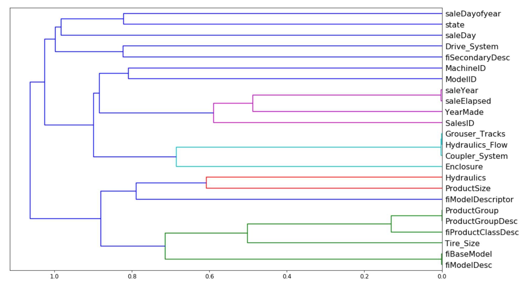
A dendrogram is based on the rank correlation of the different features in a model. It can be used to identify which features are similar (based on their rank correlation) and could likely be removed from the model. Here's an example from the second notebook:
Partial Dependence Plots
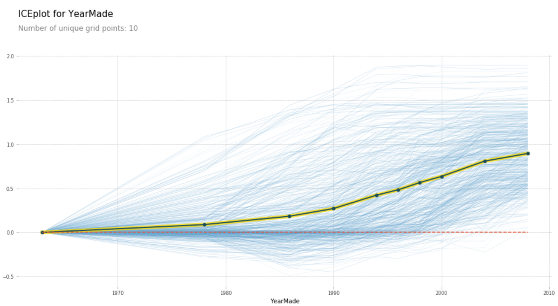
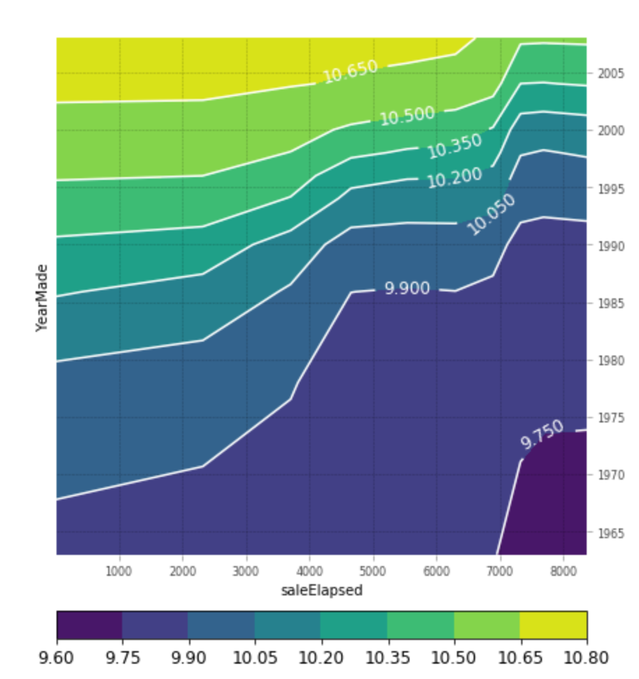
Partial dependence plots show how varying one or two independent variables affect the dependent variable. They are obtained by holding all except for one or two variables fixed and varying the remaining variables from the minimum to their maximum values. Here are two examples of such plots`:
Extrapolation
One thing random forests cannot do is to extrapolate data, i.e. make predictions for dependent variable which are outside of the training data that the random forest has been trained on. This is because a random forest is basically a stepwise approximation function. One way of dealing with this is to identify the variables which will fall outside of the training set (e.g. dates) and to mitigate the depencence on this data, e.g. either by deleting the features or capturing their content via feature engineering (e.g. include a linear trend as a feature).
Building Random Forests from Scratch
Build a simple but correct random forest implementation from scratch in python.
This creates two classes, DecisionTree and TreeEnsemble.
TreeEnsemble builds an ensemble of DecisionTrees (=the random forest).
The constructor creates n decision trees via the create_tree method.
create_tree randomly selects a number of rows from the dataset to hand
to each tree and creates n DecisionTrees, storing them in an instance variable
predict calls the predict function of all trees and averages the result.
DecisionTree recursively builds a decision tree, storing the variable
to split on, the split point, the predicted value (mean), the score as well as the left and right sub-trees (which are again DecisionTrees). It uses the find_varsplit and find_better_split to do so. find_varsplit is the
higher-level method, it iterates over all features and looks for a better
split using find_better_split for each feature. If the DecisionTree
is not a leaf it then creates left and right DecisionTrees. To avoid copying
the data, it identifies the indices that the left and right trees should
process and hands those to the child trees so that the children can use
views instead of copying the data. find_better_split iterates over all
values for a given feature in order and tries all split points to see if
they improve the overall error (which is the sum of the two errors weighted
by the datapoints for each sight). The predict method checks if the decision
tree is a leaf and returns the nodes value (=the mean of its datapoints) if
it is, otherwise it checks if the item to predict is left or right of the
nodes split point and returns the prediction of the left or right child,
accordingly.
2. Neural Nets
MNIST dataset
The dataset we work with is the MNIST dataset of handwritten numbers, first we see how to obtain and load and visualize this dataset.
Data Normalization
For neural nets (really for all linear models), it is important to normalize the data, so that all features are on a similar scale. This is important so that the gradients in gradient descent are not of completely different sizes which would lead to numerical instabilities.
Be sure to normalize all data in the same way! I.e. when using the mean and standard deviation of the training data to normalize the training data, use those same numbers to normalize the validation data (not the mean and std of the vaildation data)!
Neural Networks
A neural network is an infinitely flexibile function (general approximation theorem) consisting of layers. A layer is a linear function, such as matrix multiplication followed by a non-linear function (the activation).
In pytorch, we can define a model as follows:
import torch.nn as nn

net = nn.Sequential(
    nn.Linear(28*28, 100),
    nn.ReLU(),
    nn.Linear(100, 100),
    nn.ReLU(),
    nn.Linear(100, 10),
    nn.LogSoftmax()
).cuda() # .cuda() means run on GPU
Logisitic Regression with Neural Nets and PyTorch
A logistic regression can be implemented with a neural net in pytorch as follows:
def get_weights(*dims): return nn.Parameter(torch.randn(dims)/dims[0])
def softmax(x): return torch.exp(x)/(torch.exp(x).sum(dim=1)[:,None])

class LogReg(nn.Module):
    def __init__(self):
        super().__init__()
        self.l1_w = get_weights(28*28, 10)  # Layer 1 weights
        self.l1_b = get_weights(10)         # Layer 1 bias

    def forward(self, x):
        x = x.view(x.size(0), -1)
        x = (x @ self.l1_w) + self.l1_b  # Linear Layer
        x = torch.log(softmax(x)) # Non-linear (LogSoftmax) Layer
        return x
To implement our own pytorch model, we just need to derive from torch.nn.Module
and implement the forward method. This simple model is just a linear layer
followed by log-softmax.
Why is this Logistic Regression?
One thing that isn't really explained in the course is why this is actually equivalent to logistic regression. Focusing on binary logistic retression, we're trying to predict two classes, \(0\) and \(1\):
\[ \begin{aligned} P(Y=1|X;\theta) &&=h_\theta(x) &= \frac{1}{1+\exp(-\theta^Tx)} \\ P(Y=0|X;\theta) &= 1 - P(Y=1|X;\theta) &=1-h_\theta(x) &= \frac{\exp(-\theta^Tx)}{1+\exp(-\theta^Tx)}, \end{aligned} \]
where \(\theta^Tx = w^Tx + b\). Given observations \((x,y)\), we find the best parameters \(\theta\), by maximizing the likelhood function
\[ \begin{aligned} L(\theta|x) &= P(y|x;\theta) \\ &= \prod_i P(y_i|x_i;\theta) \\ &= \prod_i h_\theta(x_i)^{y_i}(1-h_\theta(x_i))^{1-y_i} \\ \end{aligned} \]
This is equivalent to minimizing the negative log-likelihood function
\[ \begin{aligned} -\log(L(\theta|x)) &= -\log(P(y|x;\theta)) \\ &= -\sum_i \log(h_\theta(x_i)^{y_i}(1-h_\theta(x_i))^{1-y_i}) \\ &= \sum_i -y_i\log(h_\theta(x_i)) - (1-y_i)\log(1-h_\theta(x_i))\\ \end{aligned} \]
In the neural net, we have the linear layer \(w^Tx + b\) followed by the softmax function \(\frac{\exp(x)}{\sum_{i}\exp(x_i)}\) followed by the loss function \(-y\log(p) - (1-y) \log(1-p))\). Putting these things together, it is easy to see that they are the exact same thing and that training this model is indeed the same as doing logistic regression.
Stochastic Gradient Descent (SGD)
Gradient descent is a general function minimization framework where we look for the minium of a function by taking small steps in the direction of the negative gradient:
\[a_{n+1} = a_n - \alpha \nabla F(a_n),\]
where \(\alpha\) is the learning rate and \(\nabla F\) is the derivative of \(F\) at \(a_n\).
Stochastic gradient descent (SGD) differes from gradient descent in that it doesn't use all of the data at once. It processes the data in (mini-)batches, one batch is a small part (e.g. 64 items) of the data set. One epoch is complete once each data sample as been used once in the training loop.
The course implements making these steps in the training loops in the fourth notebook, thereby replacing a simple optimizer.
Regularization and Weight Decay
To prevent models from overfitting, we can add regularization which is an extra term of the loss function that penalizes large parameter values. Typical are \(L^1\) and \(L^2\) regularization. In the derivative of the loss function, the part comming from regularization is called weight decay.
Embedding Matrices
According to the embedding discussion in lecture 11 embeddings are basically a sparse representation of an otherwise "n-hot" encoded representation of features. *"Embedding means make a multiplication by a one-hot ecnoded matrix faster by replacing this with a simple array lookup".
I found it hard to belief that this is really all that is to embeddings, so I did some reading on the side and found this medium post to be helpful. It states:
An embedding is a mapping of a discrete — categorical — variable to a vector of continuous numbers. In the context of neural networks, embeddings are low-dimensional, learned continuous vector representations of discrete variables. Neural network embeddings are useful because they can reduce the dimensionality of categorical variables and meaningfully represent categories in the transformed space.
Neural network embeddings have 3 primary purposes:
- Finding nearest neighbors in the embedding space. These can be used to make recommendations based on user interests or cluster categories.
- As input to a machine learning model for a supervised task.
- For visualization of concepts and relations between categories.
So in summary, for me embeddings are learned, low-dimensional representations (compared to 1-hot encoded, anyway) of categorical variables. The big questions is how to learn these embeddings.
I know seem to get what Jeremey means - if a categorical variable has a certain feature, it will select (array-lookup) a row from the embedding matrix - the weights in the embedding matrix will be learned.
There is also a paper discussed on the embedding approach to the Rossmann challenge winning third place in the competition. and the corresponding code.
There is more discussion of this approach with a few tips:
- When using embeddings, treat variables as categorical where possible (i.e. when the cardinality is not too high).
- Think about limiting the cardinality (e.g. "open for months" was limited to 24 months or more).
3. Practical Advice
Throughout the lectures, there are quite a few pieces of practical advice. This is maybe the most important and valuable part of the course and something that is less present in other courses. Here are my most important take aways:
How to learn
You learn by (a) doing things and (b) explaining them, so
- Apply everything you learn to practical problems, e.g. Kaggle challenges and
- Write blogposts / kaggle kernels from the very beginning
Generalization and Validation Sets
The most important question in machine learning is does it generalize, i.e. does a model trained on training data also perform well on data that it hasn't seen. To test this the most important idea in machine learning is to split the training data into a training set and a validation set. The training set is used to train the model, the validation set is used to test the trained model with the goal to see if the model performs well on data that it hasn't seen.
It is important that the validation set is differs from the test set in the same way as the future data that the model will work on differs from the training data. Therefore, randomly sampling the validation set from the training data maybe inadequate if the unseen data that the model will work on is not the same as the data that the training set is from. For example, if we want to predict store sales for the next six week, the validation set could be the last six weeks of the training data, not a random sample.
Another way to check in Kaggle competitions if the validation set is a good predictor of test set results is to plot the validiation and test set scores of different models on a scatter plot. They should fall (approximately) on a line, in this case the performance on the validation set is a good predictor of the performance on the test set.
One way to test if the validation / test set is different from the training set is to see if we can predict it: label data in the validation set with 1, data in the training set with 0 and train a classifier. Can the classifier predict what data is in the validation and what is in the training set? If so, which features does it use to predict this? Can we make the model independent of these features?
Subsample to go Fast
When exploring data, its imortant to keep things fast to be able to experiment interactively. Subsample the data if it is too large to make sure that things are fast and responsive.
Overparameterize, then Regularize
In classical statistics, people tried to use the smallest models possible in order go get better generalization results. According to Jeremy, in modern machine learning it is better to overparameterize (i.e. use a model with lots of parameters) and to use regularization to prevent overfitting.
4. NLP / Sentiment Analysis
To dip the toes into NLP, the last few lectures spent a bit of time doing sentiment analysis on an IMDB review dataset.
Tokenizing and the Term-Document Matrix
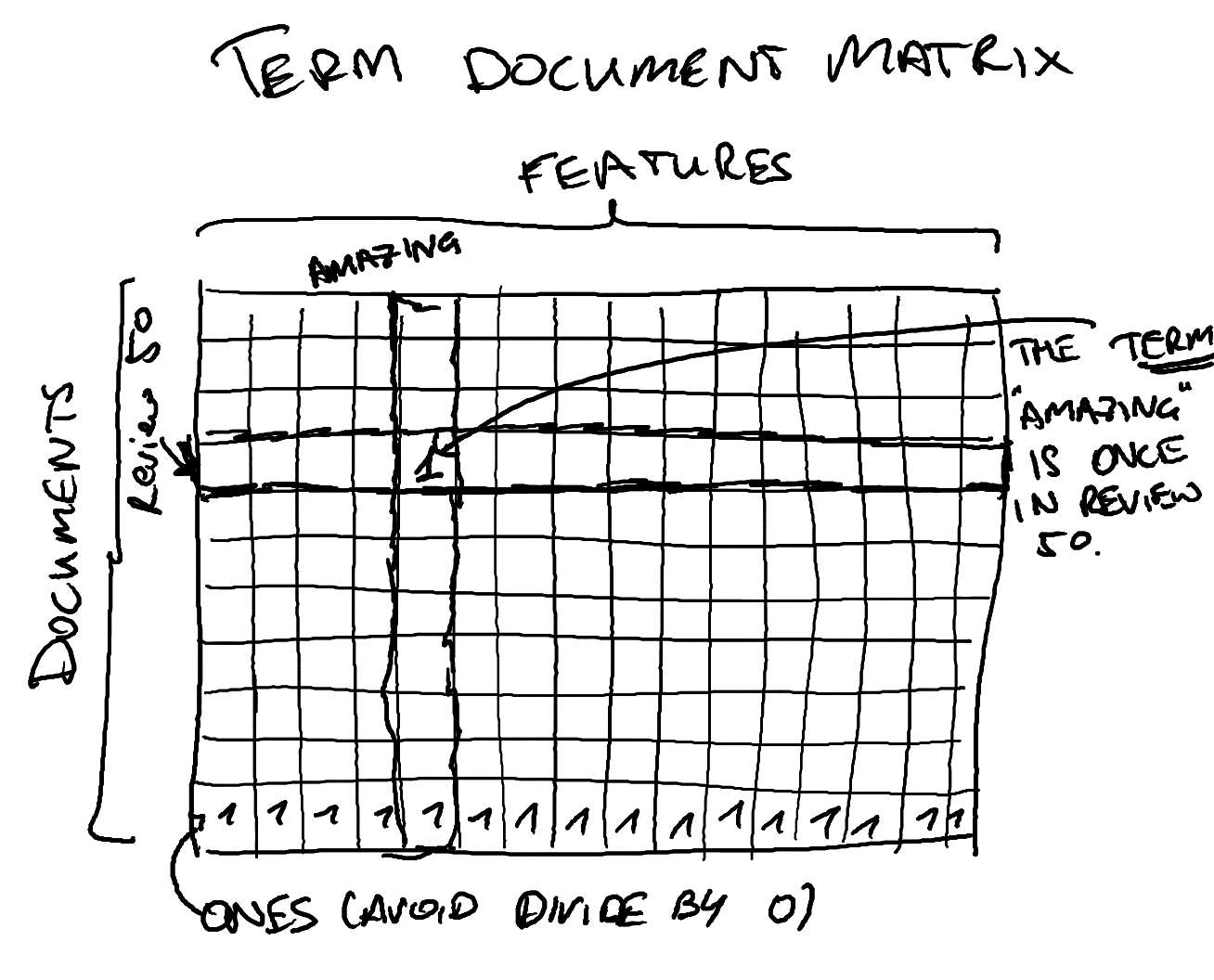
After loading the data, use scikit-learn's CountVectorizer to create a
vectorizer to create a term-document matrix which is a matrix where the
rows a documents (samples), the columns are terms (features) and the entries
are how many times a term appears in a given document. This can be used for
various ways of doing text classification.
Naïve Bayes and Binarized Naïve Bayes
The term document matrix is then used for naïve Bayes and binarized naïve Bayes classifications. The calculations for naïve Bayes are introduced very quickly without much explanation - again I feel like having to go a bit deeper to understand what is going on.
Here is the code from the fast.ai notebook:
from fastai.nlp import *

veczr = CountVectorizer(tokenizer=tokenize)

# training and validation term-document matrices
trn_term_doc = veczr.fit_transform(trn)
val_term_doc = veczr.transform(val)

def pr(y_i):
    p = x[y==y_i].sum(0)
    return (p+1) / ((y==y_i).sum()+1)

x=trn_term_doc
y=trn_y

r = np.log(pr(1)/pr(0))
b = np.log((y==1).mean() / (y==0).mean())

# Naive Bayes
pre_preds = val_term_doc @ r.T + b
preds = pre_preds.T>0
(preds==val_y).mean()
How does this work and what does it have to do with naive bayes?
trn_term_ and val_term_doc are term document matrices as
in our picture above without the one row at the bottom, so the
(i,j) entry is the number of times word j appeared in
document i.
r is a vector of the log count ratio for each feature (word),
which is computed as
\[ r(f) = \log\frac {\frac{\#\text{f in positive documents}}{\#\text{positive documents}}} {\frac{\#\text{f in negative documents}}{\#\text{negative documents}}} \]
b is the bias, here the log-ratio of positive and negative documents
\(b = \log\frac{\#\text{positive documents}}{\#\text{negative documents}}\).
For sentiment analysis, we're interested in predicting if a review is positive or negative, this is a classification task with two classes, \(1\) and \(0\).
We predict class \(1\) if val_term_doc @ r.T + b > 0 otherwise we predict
class \(0\). (@ is a new operator in python used for the matrix product here).
What this does is that for each document (row of val_term_doc) it takes all the
features (words) and multiplies them with their log-count ration and sums them
and then adds the overall bias. In other words, we predict that a document
(\(d\)) is in class \(1\) (positive) if the sum of the number of times a
word (\(w\)) appears in the document (\(d(w)\) multiplied by the words log-count ratio (\(r(w)\)) plus the bias is more than 0:
\[ \sum_w d(w) r(w) + \log\frac{\#\text{positive documents}}{\#\text{negative documents}} > 0 \]
To understand why this is indeed naive bayes classification, let's take a look at how Naive Bayes classification works. We want to know the probility of the two classes given a set of words in a document \(\vec{w}=(w_1,\ldots,w_n)\):
\[ \begin{aligned} P(1|\vec{w}) &= P(1|w_1,\ldots,w_n) \\ P(0|\vec{w}) &= P(0|w_1,\ldots,w_n) \end{aligned} \]
and we will predict the class of whichever probability is greater, so \(1\) if \(P(1|\vec{w}) > P(0|\vec{w})\) and \(0\) otherwise. Looking at the ratio this is \(\frac{P(1|\vec{w})}{P(0|\vec{w})} > 1\).
Using Bayes' rule \(\left(P(A|B) = \frac{P(B|A)P(A)}{P(B)}\right)\) we get
\[ \frac{P(1|\vec{w})}{P(0|\vec{w})} = \frac{\frac{P(\vec{w}|1)P(1)}{P(\vec{w})}}{\frac{P(\vec{w}|0)P(0)}{P(\vec{w})}} = \frac{P(\vec{w}|1)P(1)}{P(\vec{w}|0)P(0)} \]
Now the Naive part of Naive Bayes is that the probabilities of the words are all independent so that we can write \(P(\vec{w}|1) = P(w_1,\ldots,w_n|1) = P(w_1|1)\cdot \ldots \cdot P(w_n|1)\):
\[ \frac{P(\vec{w}|1)P(1)}{P(\vec{w}|0)P(0)} = \frac{P(w_1|1)\cdot \ldots \cdot P(w_n|1)P(1)} {P(w_1|0)\cdot \ldots \cdot P(w_n|0)P(0)} = \frac{P(w_1|1)\cdot \ldots \cdot P(w_n|1)} {P(w_1|0)\cdot \ldots \cdot P(w_n|0)} \cdot \frac{P(1)}{P(0)} \]
So now we want to predict class \(1\) if
\[ \frac{P(w_1|1)\cdot \ldots \cdot P(w_n|1)} {P(w_1|0)\cdot \ldots \cdot P(w_n|0)} \cdot \frac{P(1)}{P(0)} > 1 \]
Taking logarithms on both sides we get
\[ \log \frac{P(w_1|1)\cdot \ldots \cdot P(w_n|1)} {P(w_1|0)\cdot \ldots \cdot P(w_n|0)} + \log \frac{P(1)}{P(0)} = \log \frac{P(w_1|1)}{P(w_1|0)} + \dots + \log \frac{P(w_n|1)}{P(w_n|0)} + \log \frac{P(1)}{P(0)} > 0 \]
The second part \(\log\frac{P(1)}{P(0)}\) is our bias part where the probabilities are replaced by the relative number of documents:
\[ \begin{aligned} P(1) & \approx \frac{\#\text{positive documents}}{\#\text{all documents}} \\ P(0) & \approx \frac{\#\text{negative documents}}{\#\text{all documents}} \\ b & = \log\frac{\#\text{positive documents}}{\#\text{negative documents}} \\ & = \log\frac {\frac{\#\text{positive documents}}{\#\text{all documents}}} {\frac{\#\text{negative documents}}{\#\text{all documents}}} \\ & \approx \log\frac{P(1)}{P(0)} \end{aligned} \]
and the items from the first part \(\log \frac{P(w_1|1)}{P(w_1|0)}\) correspond to
\[ \log \frac{P(w_1|1)}{P(w_1|0)} \approx \log\frac {\frac{\#\text{f in positive documents}}{\#\text{positive documents}}} {\frac{\#\text{f in negative documents}}{\#\text{negative documents}}} = r(w_1) \]
Now if we assume that the same word can appear multiple times in the word vector \(\vec{w}=(w_1,\ldots,w_n)\) then we get multiple \(r(w)\) for this word, which we can summarize by multiplying \(r(w)\) by the number of times the word appears in the document (\(d(w)\)).
So yeah, the analysis in the fast.ai document is indeed the Naive Bayes classification, but it was far from obvious to me given the brevety of the presentation!
Binarized Naïve Bayes
Now binarized Naive Bayes is pretty simple from this, instead of considering if a word appears multiple times in a document, we just consider if it appears at all:
# binarized Naive Bayes
x=trn_term_doc.sign()
r = np.log(pr(1)/pr(0))

pre_preds = val_term_doc.sign() @ r.T + b
preds = pre_preds.T>0
(preds==val_y).mean()
Logistic Regression
The next step is to estimating the parameter weights not via Naive Bayes but by applying logistic regression. Using logistic regression with the binarized term document matrix improves the validation set accuracy from 0.83 to 0.884.
According to Jeremy Howard it is generally better to learn parameters than to rely on some theoretical model.
Including Bigrams and Trigrams
The next step is to not only use words but also pairs (=bigrams) and triples (=trigrams) of words. To keep the featurespace from exploding completely, Jeremy limits the features to 800.000. Applying logistic regression to these features improves accuracy further to 0.905.
Regularizing Towards Naive Bayes
The last improvements has some interesting idea of combining Naive Bayes and logistic regression. This can be found here in the video of lecture 11.
First, we replace the term document matrices by multiplying each feature count with the log count ratio (\(r\)) and then apply logistic regression to that term-document matrix. This improves accuracy once again! Here is why this works:
After fitting, logistic regression predicts \(\sigma(\beta^Tw)\), where \(\sigma\) is the logistic function, \(\beta\) is our fitted parameter vector and \(w\) is the vector of features. Based on this, it shouldn't really matter if we multiply our feature vector \(w\) with other weights before fitting logistic regression, because the logistic regression model weights \(\beta\) could simply change to undo this change. However, it does end up mattering because \(\beta\) is regularized, i.e. pulled towards 0. The log-count ratio makes some features larger or smaller and we need "less" \(\beta\) to make features count in this way. So multiplying the term-document matrix by the log-count ratios changes the features so that it is easier for a regularized model to use the features in a way consistent with the log-count ratio. This idea was first presented in the paper Baselines and Bigrams: Simple, Good Sentiment and Topic Classification as the NBSVM-bi model, which gave state-of-the-art results in 2012.
To take this insight further,
Jeremy build a learner
into the fast.ai library has a learner which actually regularizes
actively towards Naive Bayes baseline instead of 0. This improves the
result further to an accuracy of 0.922. This is contained in the
DotProdNB model in the fast.ai library.
5. Programming Python
There are also some tips and tricks and discussions on how to do things in python. Since I came to this course with decent python and scientific computing knowledge I didn't feel like I learned so much here, I'll focus on what was new-ish for me or I think is useful to come back to.
Element-wise Operations and Broadcasting
To write code that runs fast, it is important to take advantage of vectorized operations, because looping in python will be several magnitudes slower. One key approach to do this is to take advantage of element-wise operations and broadcasting. Element-wise operations expand a scalar to apply to every element of a vector, matrix or higher-dimensional tensor. Similarly broadcasting expands a smaller vector or matrix to a larger one based on the following rules:
Broadcasting rules:
When operating on two arrays, Numpy/PyTorch compares their shapes element-wise. It starts with the trailing dimensions, and works its way forward. Two dimensions are compatible when
- they are equal, or
- one of them is 1
So with two arrays a and b with a.shape = (4,3,2) and b.shape = (1,3,1),
b will be expanded to shape (4,3,2) where b is first replicated along the
third axis and then again along the first axis.
To create the right shape, we can either use the .reshape method or index using
None. Let's say b is really a 1-d array of length b = np.array([1,2,3]), we
can turn b into a (1,3,1) 3-d array either by calling b.reshape(1,3,1),
b.reshape(1, 3, -1), b.reshape(-1, 3, 1) or b[None, : , None]. When using
reshape with -1 numpy figures out the right size along that dimension.
comments powered by Disqus